
In my first blog, I provided a snapshot of global air pollution and associated health impacts. But how did scientists obtain these results? And, crucially for policy decisions: how do we think the health numbers would change if air pollution concentrations changed?
The key is to estimate an exposure-response curve (ERC), also known as a concentration-response function (CRF), a model with which we can plug in some information about an area and estimate the effects of air pollution on the people in that area. Statistical analysis allows us to develop such a model by finding, codifying, and validating patterns observed in real-world data sets.
The outcomes of interest commonly include short-term events such as deaths, hospitalizations and emergency department visits, or asthma rescue medication usage, as well as longer-term outcomes such as the prevalence of asthma, COPD, or lung cancer in an area. The input information typically includes the air pollution concentration as well as factors that could confound the relationship between air pollution and the health outcome, such as temperature, humidity, seasonality (accounting for factors such as airborne allergens and influenza rates), and socioeconomic status (SES) factors.
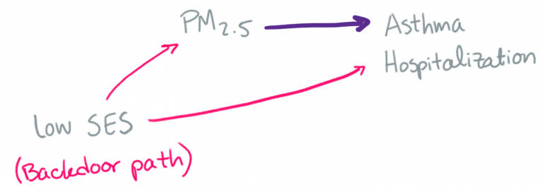
If we didn’t include these other variables, then the observed health effect of air pollution might be thrown off by the relationships between these other variables and air pollution (e.g. there’s often more air pollution at certain times of year) and between these other variables and the health outcomes of interest (e.g. there are often more deaths at certain times of year). Here’s an example DAG (directed acyclic graph), a common visualization used by epidemiologists. We’re interested in the relationship along the purple arrow, so we have to account for the relationship along the pink arrows.
Even when considering short-term health impacts, we often need to consider the air pollution (or other environmental variables) across multiple days. This is both because the health effect of air pollution from one day might not occur (or be documented) for one or more days, and because of the potential cumulative effect of air pollution across days. There are a number of techniques for analyzing these distributed lags in statistical models. Statisticians: I recommend checking out the dlnm R package!
Models get more complicated when we consider possible nonlinear relationships and effect modification. Here is an illustration of the difference between a linear and nonlinear ERC.
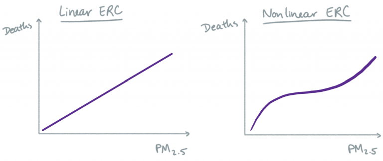
With a linear model, we are assuming that a change in air pollution will result in the same change in health outcome, regardless of what the initial air pollution concentration was. With a nonlinear model, we acknowledge the possibility that the relationship at low levels of air pollution might be different than the relationship at high or moderate levels of air pollution. GAMs (generalized additive models) are often used for estimating nonlinear relationships between environmental exposures and health outcomes. Whether a linear ERC is a realistic model for the association between PM2.5 and mortality, for example, remains an active research question.
One challenge in developing an ERC that spans the observed concentrations of an air pollutant is that many regions around the world almost never experience very high (or very low) concentrations of air pollution in modern times, and it is nontrivial to combine estimates from studies that were carried out under very different conditions, as is often the case in different countries. One widely-used integrated ERC was published in 2014.
Effect modification occurs when the level of one variable influences the ERC of another variable. For instance, the ERC of ambient ozone for people who smoke may look different than the ERC for non-smokers. Often, epidemiological analyses will investigate possible effect modification by SES, motivated by the reduced access to health information and services as well as by the plethora of pre-existing health burdens that people of lower SES commonly experience (which may also exacerbate their reaction to air pollution), including malnutrition, acute stress, and exposure to other environmental pollutants.
Often, the choice of statistical model in an epidemiologic study depends on the available data. Or, conversely, the desired form of results guides the choice of which data to use or collect (if possible). Individual-level data, which is very useful in allowing statistical control for factors such as lifestyle and pre-existing health conditions, is often not available to researchers due to data privacy concerns and/or cost of acquiring individual data. In this case, many researchers use area-aggregated measures, e.g. at the city or county level. If individual data is available, a standard modelling choice is a case-crossover analysis. If ecological (aggregate) data is used, a standard choice is a time-series analysis (2003 statistical review).
In my next blog, I will discuss air quality data availability and associated challenges.
More from Ellen Considine here.
HPHR.org was designed by ComputerAlly.com.
Visit HPHR’s publisher, the Boston Congress of Public Health (BCPH).
Email communications@bcph.org for more information.
Click below to make a tax-deductible donation supporting the educational initiatives of the Boston Congress of Public Health, publisher of HPHR Journal.![]()